Using textures as render targets
In numerical computations, the numerical algorithms are often separated from the visualizations. Sometimes, these results need to be used in other computations and not all the computational results are suitable for visualization or even at times are not of direct interest to be analyzed. Hence, directly drawing the results to a canvas is not really the most elegant solution.
Textures are the go-to data-structures to represent the solution domains in Abubu.js applications, and to store data and transfer data between different Abubu.Solvers.
We will explain this program by modifying the Julia Set application which we developed in the previous example.
Here, we will define a Abubu.Float32Texture to store the results of our computations. To do so, we need to add the following line to the main <script> section.
var result_texture = new Abubu.Float32Texture(512,512) ;
The above line will define a 512x512 texture with the Float32 type rgba values per pixel of the texture.
The next step is to redirect the output of the solver to this texture. The definition of the solver changes to:
var julia = new Abubu.Solver( {
    fragmentShader  : source('fshader'),
    targets : {
        outcolor : { location :0, target : result_texture }
    }
} ) ;
Notice how the canvas line is removed from the Solver definition. The targets or renderTargets keyword is used to allocate the output/outputs if the solver to textures. Each solver can output several textures (usually up-to 8). Each texture can have rgba values.
The term outcolor is the name of the output in the fragment shader. Its location is a layout option that should be passed to the solver in the ascending order. This section will become more clear in the next tutorials and the target is the handle to the texture that we want to attach to this output.
Now, when we render this solver, the output will be automatically stored in this texture.
We modify the fragment shader include more detail as the output about how the series diverged. In studying fractals, this is usually known as the coloring scheme of the fractal. We have implemented a simple one based on the number of iterations that we could finish and the modulus of the complex number in the sequence when the condition of \(|z|<2\) was breached or when the loop was finished. The resulting shader will be:
#version 300 es
precision highp float ;
precision highp int ;

out vec4 outcolor ; /*  output of the shader
                        pixel color             */
in vec2 cc ;        /* input from vertex shader */

#define csqr(z)     vec2((z).x*(z).x-(z).y*(z).y,2.*(z).x*(z).y)

// Main body of the shader
void main() {
    vec2 z = cc*4. - vec2(2.,2.) ; /* Initial coordinate based
                            on pixel position */
    vec2 c0 = vec2(-.9,0.) ;   /* the constant c0 */

    float iter ;

    /* Iteration loop to march the iterative map for a 1000 times */
    for(int i=0; i<1000; i++){
        iter = float(i) ;
        /* the Julia map */
        z = csqr(z) + c0 ;

        if (length(z)>2.){  /* if the point is not part of the set
                                break the loop */
            break ;
        }
    }
    // Output the result in the red channel of the output
    outcolor = vec4(iter - log(log(length(z)))/log(2.),0.,0.,0.) ;
    return ;
}
That is all good, but, the information is now stored in a texture after rendering which needs to be visualized. Hence, we need to have a Solver for visualizing our texture. Abubu.Plot2D is a visualization solver that can easily visualize any of the channels in the texture with appropriate colormaps of choice. Let's jump into setting it up:
var plot = new Abubu.Plot2D({
target : result_texture , /* the texture to visualize */
channel : 'r', /* the channel of interest:
can be : 'r', 'g', 'b', or 'a'
defualt value is 'r' */
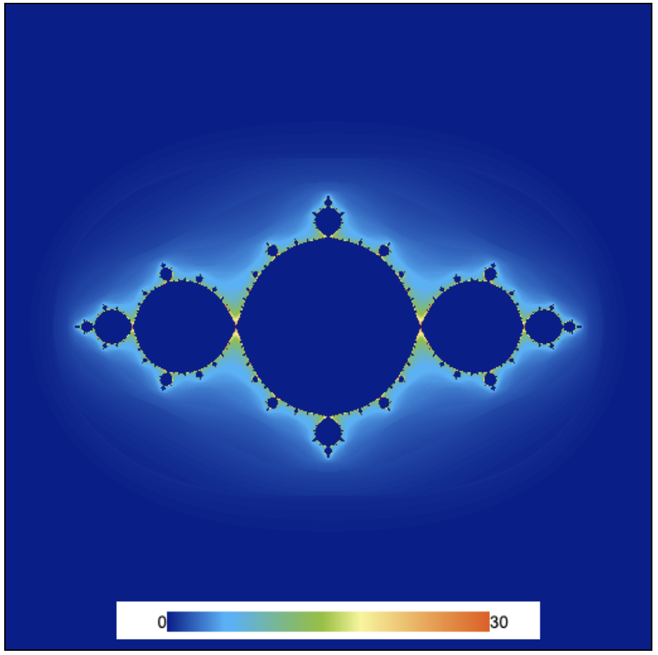
minValue : 0 , /* minimum value on the colormap */
maxValue : 30 , /* maximum value on the colormap */
colorbar : true , /* if you need to show the colorbar */
canvas : canvas_1 , /* the canvas to draw on */
}) ;
plot.init() ; /* initialize the plot */
Additionally, we make a function to solve and visualize the set at once:
function solveAndVisualize(){
    julia.render() ;
    plot.render() ;
}
At the end, we just need to call the above function to solve and visualize the set. Running the program will produce the picture below.